Projective Geometry and Transformations of 2D

“Algebra is the offer made by the devil to the mathematician. The devil says: “I will give you this powerful machine, and it will answer any question you like. All you need to do is give me your soul: give up geometry and you will have this marvellous machine.” . . . the danger to our soul is there, because when you pass over into algebraic calculation, essentially you stop thinking: you stop thinking geometrically, you stop thinking about the meaning.” - Sir Michael Atiyah

This is first in a series meant to go through some of the chapters in Hartley and Zisserman’s book titled Multiple View Geometry in Computer Vision. A cursory preview can be found in this earlier post. This post covers the first part of Chapter 2 in the aforementioned book.

Preamble

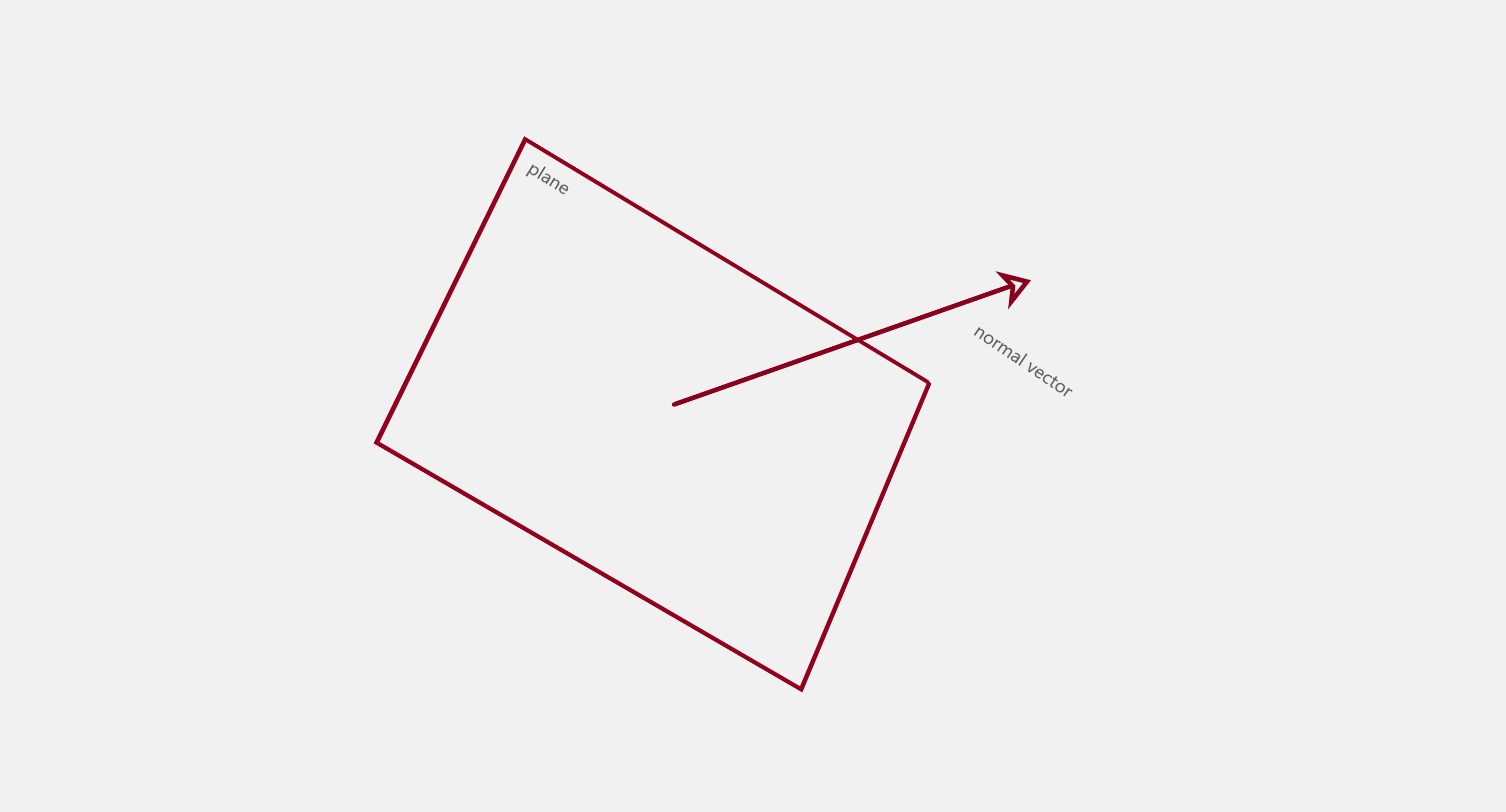
In this series, we will be looking at the geometric and algebraic principles used to analyze and understand spatial relationships between objects in space. I believe it’s always helpful to remember that this journey takes us through a very illuminating map of spatial objects and elements. However, it’s important to note that the map is not the territory, and a description of a square is not the square itself, but rather a rich view that encodes the characteristics of that square. For example, a plane is represented mathematically by its normal vector, this method references the fact that we can represent a set by an element that is not contained within it. As an example of this, let’s consider that you have 5 out of the only 6 cars that exist in the world, you can represent your cars by listing all the cars that you have, but if you want to conserve time and space, you can as well represent your cars by listing the only car that you do not have, thus, the exception determines the rule.

First, let’s get through some basic ideas.

• A model is a description or characterisation of an element, and that description serves as a window through which we may view a particular set of features possessed by the element under consideration, we know that no model is absolute, so a combination or fusion of models supplies a richer view of the peculiarities and particulars of that element.

• Euclidean Geometry was seen as the only geometry, as it described the visible space we live in to great exactness. Then it was believed that the parallel postulate was such a necessary property of straight lines that it would follow from the previous postulate, however this was found to be an erroneous assumption, the parallel postulate does not arise from the first 4 and is not superfluous, this means that if we take the first 4 to be true, it does not necessarily mean that the 5th is false or true. And since we cannot travel to infinity to verify the case ourselves, the consequence is that we can assume the parallel postulate to be true or false, and based on the varying interpretations, we get different types of geometry (different descriptions of space), this means there can be more than one logically possible geometry.

• Equality between entities/objects mainly specifies and refers to those components that are identical, which may only be part of an entity but determine the whole, and specify its intrinsic meaning, as determined by the intentions used to characterise the entity. When we say that entities are identical to each other, they may not be the same, but they share the same properties with respect to all the operations we expect to perform on it. For example, am I the same as the person I was yesterday? perhaps not, but am I equal to that person for all legal intent and purposes? yes I am…within the space of physiological/philosophical operations, I may not be equal to who I was yesterday, but within the space of legal operations, I am ‘legally equal’ to that person as a legal entity.
  

Our focus is primarily on projective geometry, but to gain a good foothold, we need to set our feet on more solid ground, and sweep through the basic ideas.

The 2D Projective Plane

When I use the word geometry, these are the terms that go through my mind, each progressively expanding on the previous.

• Geometry is the study of shapes and their properties
• Geometry is the study of figures on a surface and their properties
• Geometry is the study of figures on a surface and the spatial qualities that distinguishes it from other figures.

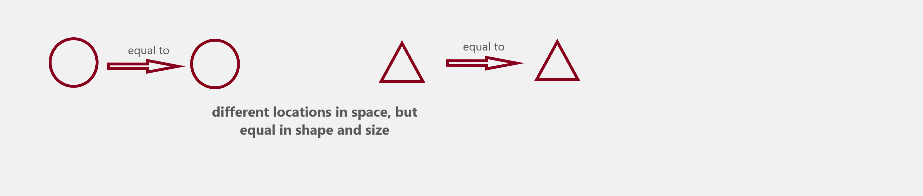
We can determine the spatial qualities that make a shape distinguished, by identifying those properties that make it equal to another instance of the same shape. Hence if two squares are equal, then they share the same properties…likewise, if they share the same properties, then they are equal. What makes a square equal to another square? We can say two squares are equal if placing one atop the other creates an identical match in shape and size…the notion that we need to place one shape atop the other informs us that there is some kind of motion taking place. Hence, two shapes are equal if there exists a motion that superimposes the first object on the second so that they match each other exactly in shape and size. Now if the objects are the same, before and after such a transformation, identical properties must remain the same, so we can say that any spatial property that is preserved when you subject that object to a transformation from itself to an identical object of same shape and size but different location is a geometric property of the object. (i.e I remain the same person to who I was before I walked across a room).

Since, we can specify, describe and observe objects through their properties, geometry can be succintly described as the study of invariants (set of geometric properties that do not change) under a set of transformations (a group of select motions). This idea of relating properties of figures to the associated geometry was introduced by Felix Klein (1849-1925).

Here we distinguish between two kinds of transformations - rigid motion and projection

Metric: A rigid motion effects a change in the position of an object in space through rotation and translation. A geometric property which is preserved by all rigid motions is a metric property (distance, angle, area etc), a theorem that deals with metric properties is a metric theorem, and Euclidean geometry is the geometry of metric properties inclusive of the metric theorems.
Projections: A property that is preserved by all projections is called a projective property (that a curve be a straight line, that a curve be a conic etc), and the associated geometry deals merely with projective properties (invariants with respect to projection).

In summary, if 2 objects are the same, then they share the same geometric properties, that means translation from the first to the second object’s position must mean that the geometric property remains the same before translation..it must be invariant, because if the two bodies are the same, and the property changes after the relocation of one to the other body’s location, it means that the propery is not shared by both bodies in resting state (that’s why it had to change)…and it means that the property does not capture “equality” (since we originally said both bodies are equal to each other).

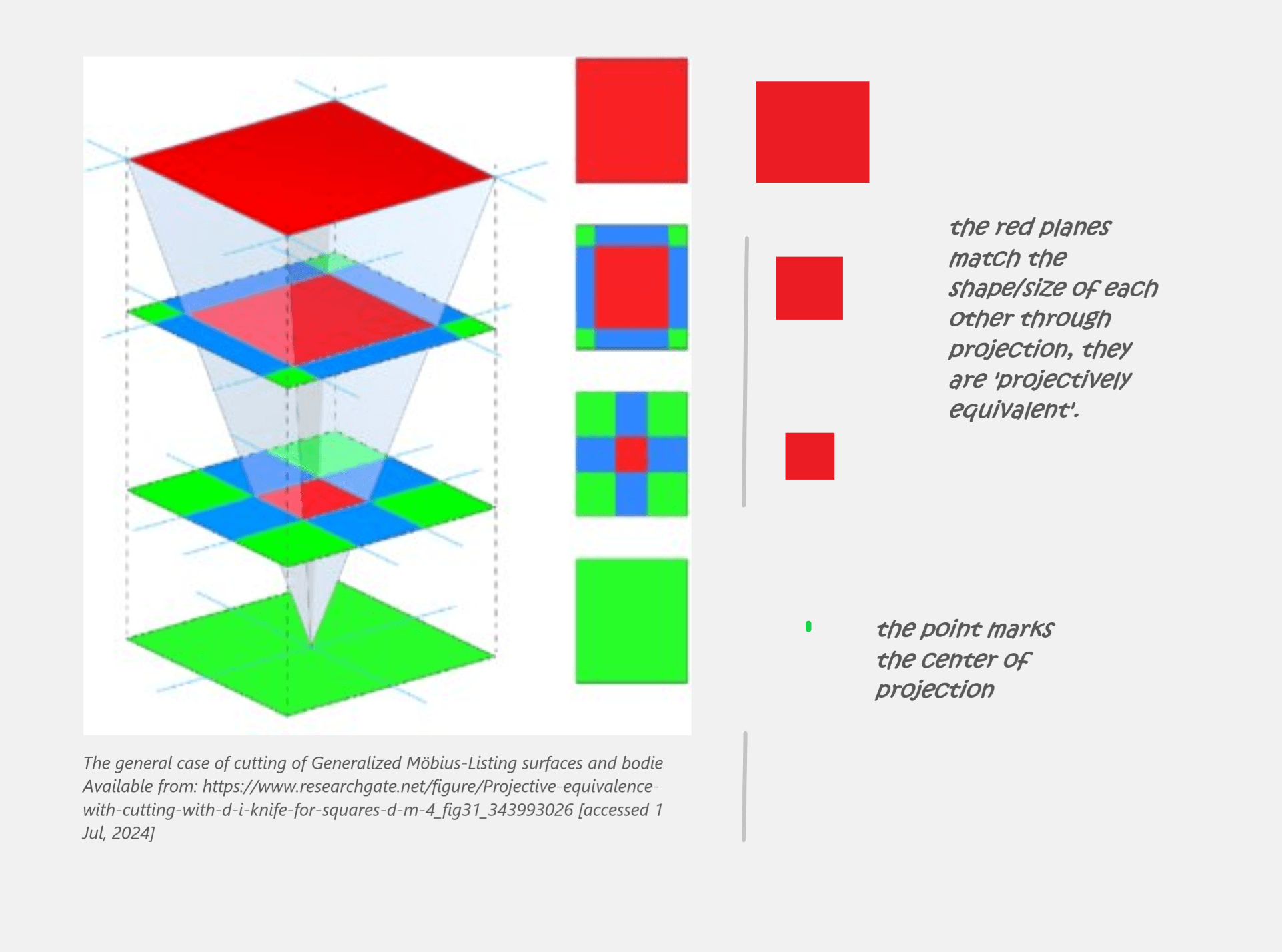
Projective Equivalence: Pursuing the above ideas further, if there exists a group of transformations that can projectively map/transform an object (points, lines etc) to take the shape and size of the other object we see both objects as projectively equivalent and we represent them (algebraically) with homogeneous coordinates (more on this later).

Time to dive into the major points of the book! - Multiple View Geometry

Planar Geometry

The book takes an hybrid approach - the algebraic and the geometric, where points and lines are described as vectors, and this leads to ease in computation.

Let’s take a look at an example

Imagine we had vectors living on a line (born in 1D space); we focus particularly on 2 vectors - on the 1-D plane shown below…and we can translate both points to any other point on the 1D number line.? The line may be oriented in various ways, but it still refers to the same 1D space. The 2 vectors only understand and live in the 1D space, you can move the 1D space around, and spin it about, put it in a box, or take it to the moon, the vectors inside that 1D space only know about the internal properties of the space they live on, all they know is that they live on a 1D conveyor belt and that conveyor belt moves them from one point to the other. They live inside a house and understand the interior alone, and do not know if the house itself has been moved or relocated to some other spot.

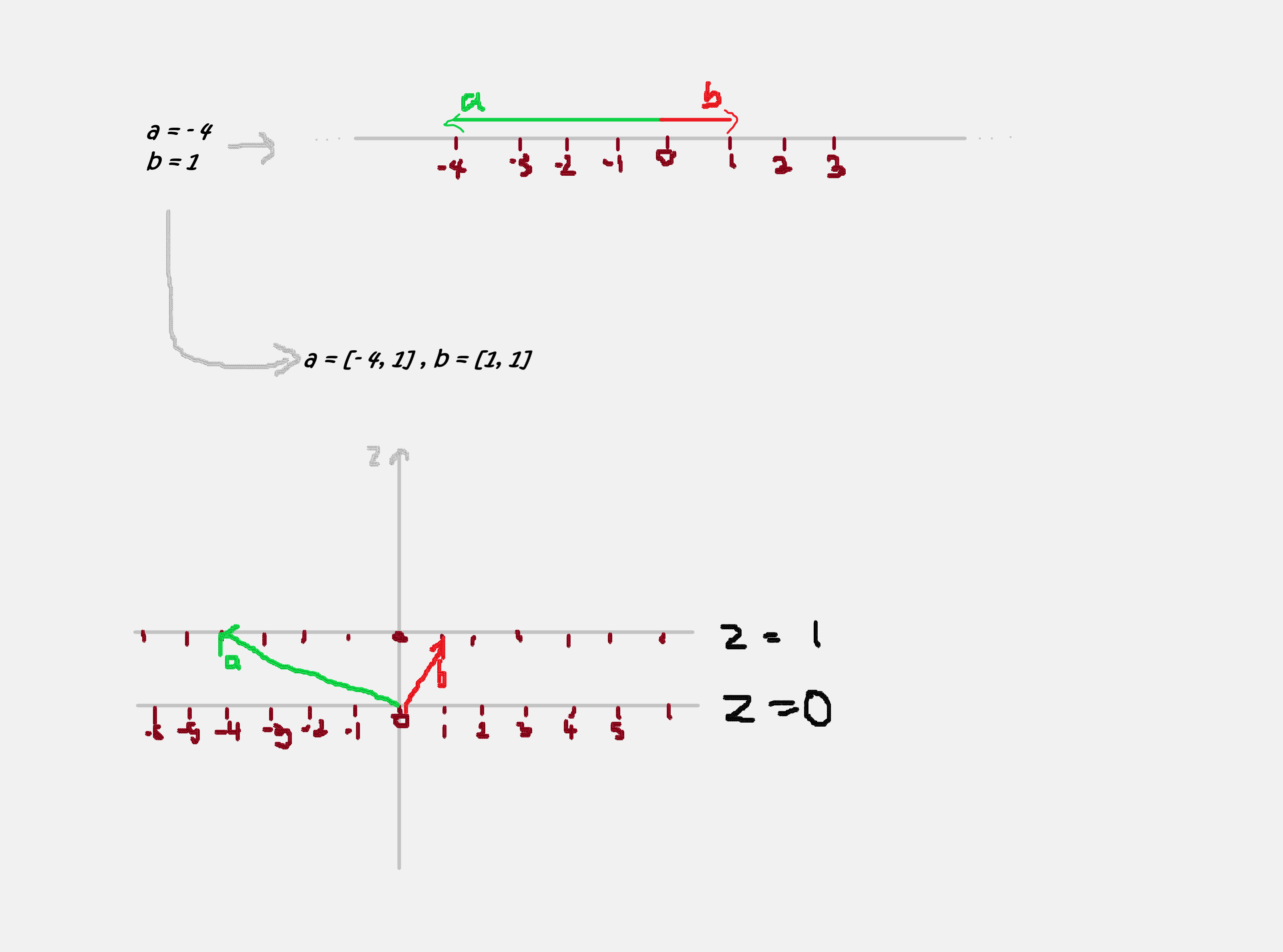
Now when both vectors are transformed, they both intend to maintain a distance between each other, let’s say the intend to maintain their current separation of 3 and we want to transform the red vector to -7, we cannot simply add -3 to the vectors because -3 is a scalar and you do not add scalars to vectors (remember that a scalar has no sense of direction and our 1D vector is oriented in a very particular way), so we need to stretch/scale the specific vector (Red) to another point on the same line, recall that we can scale or stretch via multiplication.

We can scale Red by a scaling factor, then scale blue with another scaling factor so they maintain that separation distance but how can we do this at once without having 2 different scaling factors? Well, we can use our powers of 2D and draft in a second basis vector. The factors and vectors involved in the scaling becomes 2D. We simply manipulate the vectors through 2D, and a single scaling factor. We move these vectors in 2D with a single transformation of the two basis vectors, they only see what happens in 1D, they are scaled accordingly, and are happy. So what happened? Both vectors still live in (and only have knowledge of) 1D space, so they do not know that their world has been rocked and a second dimension has been added via another basis vector…but it doesn’t matter, they do not need to know as their lives do not change (from their view). To maintain the illusion, we move them up the second basis vector by 1, so their new coordinates (in our view) become 2D, but they co-exist just the same way they did in 1D. Imagine you had a plate of food on a table, and your only reference point is that table, now someone comes in and moves the table to the other room without touching the food…nothing has changed with respect to the plate of food and that reference point - the table.

If you were to move the location of the 1D line up in the second dimension, you get the same 1D separation between the vectors, nothing between them has changed, but now you have extra levers to pull because you have an extra basis vector, the 1D space sits on the basis vectors, and if you change the x coordinate of the second basis vector, you can shift the whole space all at once, because you are basically shifting the vectors that rely on that vector as their basis. This gives us a way to reliably translate the whole 1D space, by simply shifting the basis on which the space sits on. Recall again that for all intents and purposes, the fact that red and blue are now represented as 2d vectors changes nothing about the relationship between them, in relation to each other they remain 1D vectors on that space, and you can discard the last coordinate without any adverse effects. This introduces the concept of homogeneous coordinates, where an extra dimension is brought in to give us an added lever of manipulation. We have our 1D vectors but we manipulate them in 2D, and the same goes for 2D to 3D, they live in 2D, but are manipulated in 3D…and so on it goes.

---

Now that we’ve seen that we can represent points as vectors, we recognise the fact that we can likewise represent lines as vectors. To draw a line in the plane, we generally use the equation of a line: $ax + by + c = 0$, with $x,y$ as points over the plane, $a,b,c$ determines a unique line. Points: We can represent the points as vectors in the plane $(x,y)$…hence in homogeneous coordinates, this will be $(x,y,1)$, or more generally $k(x,y,1)$ -> $(kx, ky, k)$. With $(kx, ky, k)$, if we want the exact points we started out with in Euclidean space (because Euclidean space selects a particular plane out of all equivalent planes), we divide by k so that the last coordinate value equals 1 (recall what we said in the preamble about projective equivalence and note that these points $(x,y,1), (kx, ky, k)$ are projectively equivalent).

Lines: Let’s take a look at how homgeneous lines will look like, we observe that the whole pattern forms a plane, this means we can represent our 2D lines homogeneously with a 3 vector which is normal to that plane, and this naturally turns out to be our vector $a,b,c$ from $ax + by + c = 0$. The general form of a plane : $Ax + By + Cz = D$, where $z = 0$, $Ax + By + D = 0$, (D can be any number, negative or positive).

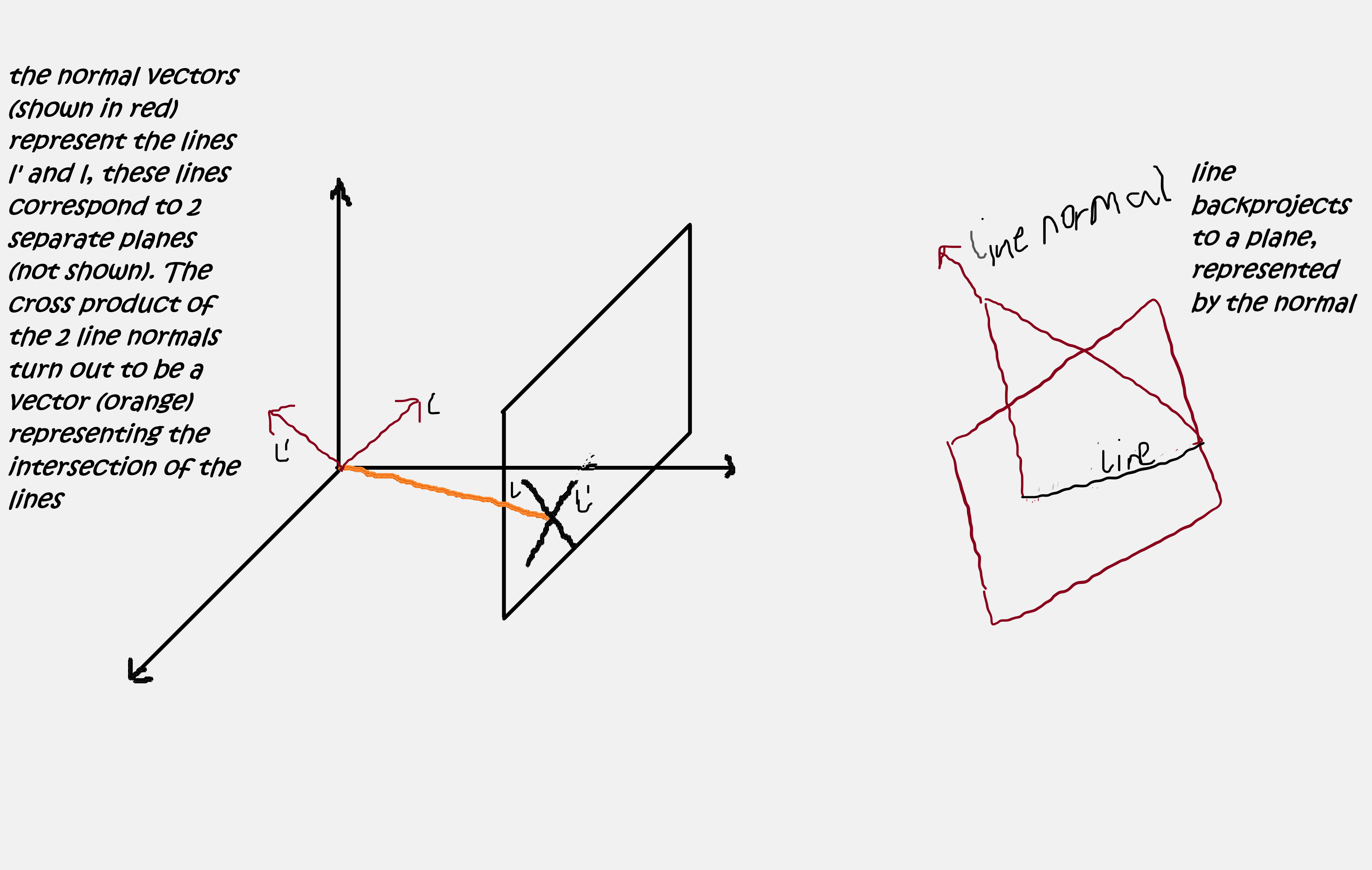
Here comes something lovely, if $(a,b,c)$ and $(x,y,1)$ are vectors ,we can insert them into the line equation to see the constraint that the dot product of the 2 vectors must be equal to 0, $(a, b, c) \cdot (x, y, 1) = 0$. This means that both vectors are orthogonal to each other with an angle of 90 degrees. We represent this relationship succintly with $l \cdot x = 0$ or $x \times l^T = 0$ or $l \times x = 0$

Intersection of lines: We know from common experience that 2 lines intersect at a point (even parallel lines, which we will see later on). Let’s check. Given two lines with a common intersection, we know that any point that lies on a line needs to satisfy $x \cdot l = 0$, so if we have two lines $l$ and $l’$, and a point lies on both lines,the vectors that represent the objects to satisfy the equations $x \cdot l = x \cdot l’ = 0$, this means that it is orthogonal to both lines…and this means we have to find the cross product $l \times l’$; thus the intersection of two lines $l$ and $l’$ is the point $x = l \times l’$

Lines joining points: Following a similar argument for the intersection of lines above, a line $l$ that joins two points has to satisfy $l \cdot x = l \cdot x’ = 0$, hence the vector representing $l$ has to be orthogonal to the vectors representing the points. Thus $l = x \times x’$ Degrees of freedom (dof): A point can be represented in the plane with the 2 coordinates $x$ and $y$…and hence has 2 dof , a line also has 2 d.o.f if you consider the point slope form of a line $y = -a/bx - c = mx + c$ …where the 2 parameters needed = $m$ and $c$, alternatively the two independent ratios ${a : b : c} => $a/b$; $b/c$.

N.B Don’t forget that these lines and points are represented in equations as vectors, hence whenever $l$ or $x$ is referred to in the context of an equation, think about the vectors representing them.

Ideal points and the line at infinity

Now we arrive at an interesting point - infinity. First we need to consider the notion that the 2D space we are looking at is a projection of the real world, hence the 2D plane is a projected reality. Now in this 2D Euclidean plane, parallel lines do not meet, but by now, we know that Euclidean geometry is not the only geometry that exists..perhaps what we do not see in the current 2D form exists in some other projected form? The following is an attempt to tackle the intuition behind these ideas. Imagine two intersecting lines and take note of both ends of both lines & the intersection point, now rotate one of those lines and watch the intersection point extend further out through your mind’s eye…at a certain point that intersection point gets farther and farther till infinity, then the line becomes parallel right? And just when you rotate past the point where it’s parallel, the intersection point immediatel snaps back to reappear at the other end of the line. At the point where the lines are parallel to each other, we may say the line intersects at infinity, since we observe that the further and further and further and further the intersection point goes, the ‘more parallel’ it becomes,we deduce therefore that the lines become parallel at the limit of intersection.

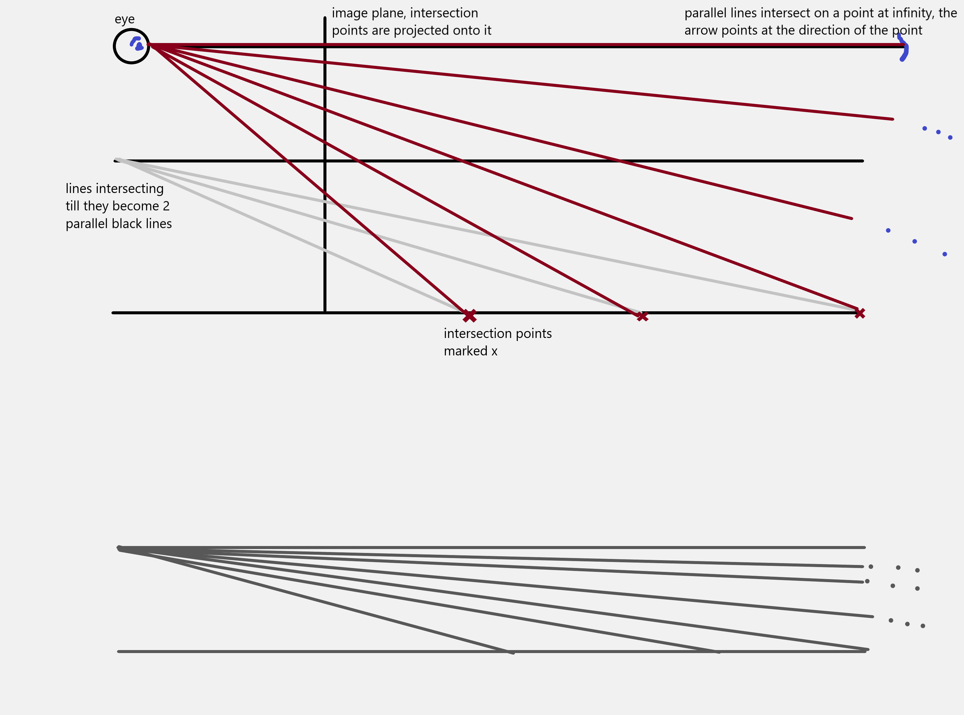
We know that we cannot play fast and loose when dealing with infinity, so we are aware of the fact that we have a point at infinity that we cannot observe, but how do we represent that point? We use vectors as usual, vectors represent direction, so even if we cannot get to that point, we can point to the ‘limiting’ direction.

Now let’s align our intuition with equations. We consider 2 parallel lines and compute their intersection points, we find that the 3rd coordinate is 0, and the inhomogeneous representation of this point (b/0,-a/0) results in a division by 0 which points to an infinitely large number $(\infty,\infty)$ and agrees with our intuition. Thus points at infinity have 0 as the z coordinate, and thus all ideal points may be represented as $(x,y,0)$. These points lie on a line (the line at infinity), and the line is represented as usual by the plane normal vector $(0, 0, 1)$

A general line $(a,b,c)^T$ intersects $l$* at the ideal point $(b, -a, 0)$ (recall how to find the point of intersection via cross product and verify with the dot product of the point and the line). The first two coordinates of this point at infinity lie on the $z = 0$ coordinate and can be as a vector that represents direction. we also notice that in inhomogeneous coordinates $(b,-a)$ is also a vector tangent to the parallel lines and orthogonal to the line normal, so we can say it represents the line’s direction.

Duality: If you can get a figure from points, and you replace each points with its dual line and you combine those points with a dual operation…the resulting figure is the dual to the initial figure.

The role of points and lines may be interchanged in these ways: -> $l^Tx = 0$ and $x^Tl = 0$ -> $x = l \times l’$ and $l = x \times x’$ What do you get when you interchange the roles of points and lines in the original theorem? What you get is the dual

For the next section we will begin with conics and dual conics

References

• Gielis, Johan & Tavkhelidze, Ilia. (2020). The general case of cutting of Generalized Möbius-Listing surfaces and bodies. 3. 7. 10.1051/fopen/2020007.

• Graustein, W. C. (1930). Introduction to higher geometry. New York, NY: The Macmillan Company.

• Hartley, R., & Zisserman, A. (2004). Multiple View Geometry in Computer Vision (2nd ed.). Cambridge: Cambridge University Press.

• Kneebone, G. T. (1960). Algebraic Projective Geometry. Oxford: Clarendon Press.